Catculator — training a 0.5M model to perform addition

Introduction

In my attempt to learn JAX, I decided to embark on this project to build an autoregressive calculator. Over a series of posts, I'll cover the following:

• data prep
• implementing a dead simple transformer
• one by one, adding components and seeing changes to loss
  • ADAM instead of SGD
  • RoPE
  • Tied embeddings
  • Masked Loss
• scaling experiments
  • data — increasing operands (9 → 99 → 999)
  • model — increasing params (0.5M → 2M → 5M → 10M)
  • operations — add, sub, multiply (no div since that introduces decimals)

With a calculator, it's easier to build intuition for how well the model is performing. With language, the model can generate plausible-sounding sequences that are still low quality. With a calculator, we can easily determine if the solution is correct, check for generalizability (test data / longer operands), and try out a variety of loss functions — token-based cross entropy, solution-based numeric penalty, etc. This gives us more room to experiment and see how the solving ability changes.

The goal of this blog is to:

• build JAX muscles
• build intuition for transformer modeling techniques and scaling
• explore profiling and performance tradeoffs

We'll start off with a notebook and slowly expand.

Generating Data

Let's start with building out the data. Since these are deterministic operations, we can generate the data with simple math operations.

The first thing we need to do is build our vocabulary that the model will learn to leverage:

vocab_list = ["#", "0", "1", "2", "3", "4", "5", "6", "7", "8", "9", "+", "-", "*", "="]

With just 15 tokens, we should be able to teach the model addition, subtraction, and multiplication. We could also try teaching it division, but that introduces the complexity of decimals and precision, so I'm leaving it out of scope for now.

We will use # as our BOS and EOS token, and we can play around with the data format — whether to pad left or right. Spoiler: it doesn't really matter, but left-padding helps standardize the T dimension to run batched inference.

To make our vocab dimension easy to work with on GPUs, we'll add a / token to round vocab_list to an even 16.

With this, we can generate our data — first as a series of string equations like 1+9=10.

Tokenizing is simple — we just iterate over the length of the sequence and map the strings to integers, leveraging numpy and vectorizing as much as possible so we can scale to 100K sequences.

A few constants we are declaring here:

• MAX_OPERAND = 99 — the maximum operand. So the max value in the data is 99+99=198.
• MAX_SEQ_LEN = 13 — the length of the padded sequence. We set it to an odd number since when we extract the ys from the sequence, we will be left with 13 - 1 = 12 in the context window.

The XY split is simple — if we have 1+1=2# as the initial sequence, then x = "1+1=2" and y = "+1=2#". So if the model sees 1+1=, the next token to predict is 2. And 1+1=2 → # to stop the calculator.

Once we tokenize the data and have a numeric matrix, we can start leveraging jax.numpy.

JAX has a clean way of allowing us to vectorize operations using jax.vmap — we'll use that to write a function for splitting a single sequence, and then apply it along the sample dimension:

def xy_split(seq):
    return seq[:-1], seq[1:]

xy_split_map = jax.vmap(xy_split)
train_X, train_y = xy_split_map(train)
test_X, test_y = xy_split_map(test)

With MAX_OPERAND = 99 we get 100 * 100 = 10k sequences. With MAX_SEQ_LEN = 13, we're looking at 10k * 13 * 1 byte (int) = 130kb of data. That's small enough to run in a single batch, but we still want to batch our data so we can easily scale to 100x when we bump MAX_OPERAND to 999.

The neat thing about JAX is that we can just add another dimension representing the batch index, and scan over that dimension — keeping all the data in one matrix rather than using generators. This assumes we can load all data into memory; perhaps this will bite us eventually.

def batchify(x: jax.Array, bs: int = BATCH_SIZE) -> jax.Array:
    N, T = x.shape
    x = x[: (N // bs) * bs]
    return x.reshape((N // bs, bs, T))

That's it on the data side. We have our basic data generated, tokenized, split, and ready to train on.

vocab_list = ["#", "0", "1", "2", "3", "4", "5", "6", "7", "8", "9",
              "+", "-", "*", "/", "="]
stoi = {s: i for i, s in enumerate(vocab_list)}
itos = {i: s for i, s in enumerate(vocab_list)}

MAX_OPERAND = 99
MAX_SEQ_LEN = 13
BATCH_SIZE  = 256
TRAIN_TEST_SPLIT = 0.72


def generate_sequence(i: int, j: int, op: str) -> str:
    if op == "+":   res = i + j
    elif op == "-": res = i - j
    else:           res = i * j
    return f"{i}{op}{j}={res}#"


def generate_data_list(max_operand: int = MAX_OPERAND) -> np.array:
    data = np.array([], dtype=np.dtypes.StringDType())
    for i in np.arange(max_operand + 1):
        for j in np.arange(max_operand + 1):
            data = np.append(data, generate_sequence(i, j, "+"))
    return data


def encode(s: str): return [stoi[c] for c in s]
def decode(t: list[int]): return "".join(itos[i] for i in t)


def encode_data(data_list_pre, max_seq_len=MAX_SEQ_LEN):
    out = np.ones((len(data_list_pre), max_seq_len), dtype=np.int32)
    for i, val in enumerate(data_list_pre):
        out[i] = encode(val)
    return out


def train_test_split(data, key=17, split_ratio=TRAIN_TEST_SPLIT):
    idx = jax.random.permutation(jax.random.key(key), jnp.arange(len(data)))
    cut = int(len(data) * split_ratio)
    return data[idx[:cut]], data[idx[cut:]]


def xy_split(seq): return seq[:-1], seq[1:]


def batchify(x, bs=BATCH_SIZE):
    N, T = x.shape
    x = x[: (N // bs) * bs]
    return x.reshape((N // bs, bs, T))


# put it all together
data_list  = generate_data_list()
data_pre   = np.strings.ljust(data_list, MAX_SEQ_LEN, "#")
data       = jnp.array(encode_data(data_pre))
train, test = train_test_split(data)
train_X, train_y = jax.vmap(xy_split)(train)
test_X,  test_y  = jax.vmap(xy_split)(test)
x, y       = batchify(train_X), batchify(train_y)
testx, testy = batchify(test_X), batchify(test_y)

Building the Transformer model

Aiming for a ~500k model, we will use these model configs:

vocab_size   = 16
d_model      = 64
num_layers   = 4
ffw_dim      = d_model * 4
num_q_heads  = num_kv_heads = 8
head_dim     = 8

Assuming tied embeddings, this gives us a total of ~590k params.

Now for the fun part — let's start by looking at all the components we need to define:

• Embedding and Unembedding layer
• Transformer layer
  • scaled dot product attention
  • feed-forward with non-linear activation
• LayerNorm
• Dropout
• RoPE (later)

Most things should be intuitive. I really like using einsum — it makes matrix multiplications declarative while handling transposing, batching, etc. neatly.

jax.jit() compiles the model into XLA, which intelligently fuses operations to avoid HBM round-trips. There are a few tricks worth leveraging to keep compile times sane:

• Transformer stack — a Python for loop over num_layers gets unrolled during compilation, so the compiler re-emits artifacts for every layer. If we use jax.lax.scan instead, we compile the transformer_layer only once.
• Across batches — the same principle. We can keep the model and data on-device and loop over batches with scan instead of returning to the host between steps.

from typing import NamedTuple

class AttentionParams(NamedTuple):
    W_q: jax.Array; W_k: jax.Array; W_v: jax.Array
    W_o: jax.Array
    W_fin: jax.Array; W_fout: jax.Array

class ModelParams(NamedTuple):
    W_embed: jax.Array
    attention_params: AttentionParams
    W_unembed: jax.Array


def init_model(seed=17):
    keys = jax.random.split(jax.random.key(seed), 10)
    n = lambda k, shape, fan_in: jax.random.normal(k, shape) / jnp.sqrt(fan_in)

    W_embed   = n(keys[0], (vocab_size, d_model), vocab_size)
    W_q       = n(keys[1], (num_layers, d_model, num_q_heads,  head_dim), d_model)
    W_k       = n(keys[2], (num_layers, d_model, num_kv_heads, head_dim), d_model)
    W_v       = n(keys[3], (num_layers, d_model, num_kv_heads, head_dim), d_model)
    W_o       = n(keys[4], (num_layers, num_q_heads * head_dim, d_model),
                  num_kv_heads * head_dim)
    W_fin     = n(keys[5], (num_layers, d_model, ffw_dim), d_model)
    W_fout    = n(keys[6], (num_layers, ffw_dim, d_model), ffw_dim)
    W_unembed = jax.random.normal(keys[7], (d_model, vocab_size))

    return ModelParams(
        W_embed,
        AttentionParams(W_q, W_k, W_v, W_o, W_fin, W_fout),
        W_unembed,
    )

def embedding_layer(x, params):   return params.W_embed[x]
def unembedding_layer(x, params): return jnp.einsum("btd,dv->btv", x, params.W_unembed)

# placeholder — replaced by real RoPE below
def rope(x): return x


def sdpa_layer(x, params):
    q = jnp.einsum("btd,dqh->btqh", x, params.W_q)
    k = jnp.einsum("bsd,dkh->bskh", x, params.W_k)
    v = jnp.einsum("bsd,dkh->bskh", x, params.W_v)

    q, k = rope(q), rope(k)

    B, T, Q, H = q.shape
    _, _, K, _ = k.shape
    groups = Q // K
    q = q.reshape((B, T, groups, K, H))

    scores = jnp.einsum("btgkh,bskh->bkgts", q, k) / jnp.sqrt(H)
    causal = jnp.where(jnp.tril(jnp.ones_like(scores)), 0.0, -jnp.inf)
    weights = jax.nn.softmax(scores + causal, axis=-1)

    out = jnp.einsum("bkgts,bskh->btkgh", weights, v)
    out = out.reshape(B, T, groups * K * H)
    return jnp.einsum("bth,hd->btd", out, params.W_o)


def ffw_layer(x, params):
    x = jnp.einsum("btd,df->btf", x, params.W_fin)
    x = jax.nn.gelu(x)
    return jnp.einsum("btf,fd->btd", x, params.W_fout)


def layer_norm(x, eps=1e-5):
    mean = jnp.mean(x, axis=-1, keepdims=True)
    var  = jnp.var(x,  axis=-1, keepdims=True)
    return (x - mean) / jnp.sqrt(var + eps)


def transformer_layer(x, params, key, is_train=True):
    k_attn, k_ffw = jax.random.split(key)
    x = x + dropout(sdpa_layer(layer_norm(x), params), k_attn, is_train=is_train)
    x = x + dropout(ffw_layer(layer_norm(x),  params), k_ffw,  is_train=is_train)
    return x

def forward(params, x, key, is_train=False):
    x = embedding_layer(x, params)
    num_layers = jax.tree.leaves(params.attention_params)[0].shape[0]
    layer_keys = jax.random.split(key, num_layers)

    def step(x, layer):
        layer_params, layer_key = layer
        return transformer_layer(x, layer_params, layer_key, is_train), None

    x, _ = jax.lax.scan(step, x, (params.attention_params, layer_keys))
    return params, unembedding_layer(x, params)

Experiments

Stochastic Gradient Descent

We start with plain SGD to see how it works out of the box. It's relatively simple to implement in the train_step with no extra args.

Running for 300 epochs with learning rate between [3e-4, 1e-3].

def loss_fn(params, batch, key, is_train=False):
    x, y = batch
    _, logits = forward(params, x, key, is_train)
    logp = jax.nn.log_softmax(logits, axis=-1)
    nll  = -jnp.take_along_axis(logp, y[..., None], -1).squeeze(-1)
    return nll.mean()


@jax.jit
def train_step(carry, batch, lr=3e-3):
    params, key = carry
    key, subkey = jax.random.split(key)
    loss, grads = jax.value_and_grad(loss_fn)(params, batch, subkey, is_train=True)
    params = jax.tree.map(lambda p, g: p - lr * g, params, grads)   # ← raw SGD
    return (params, key), loss


def eval_step(carry, batch):
    params, key = carry
    return (params, key), loss_fn(params, batch, key, is_train=False)


def train(params, x, y, epochs=100, key=None):
    if key is None: key = jax.random.key(0)
    for i in range(epochs):
        key, epoch_key = jax.random.split(key)
        (params, _), loss = jax.lax.scan(train_step, (params, epoch_key), (x, y))
        eval_loss = jax.lax.scan(eval_step, (params, key), (testx, testy))[1]
        print(f"epoch {i}  train={loss.mean():.4f}  test={eval_loss.mean():.4f}")
    return params

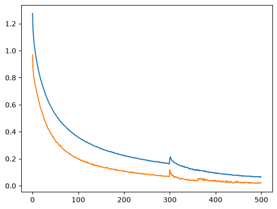
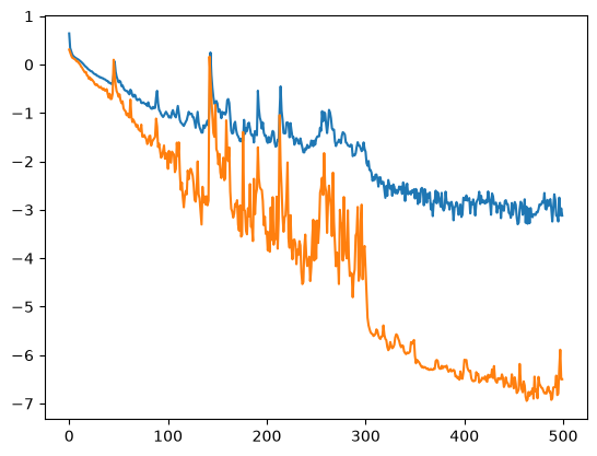
We get to a train and validation loss of 1.16 and 1.04 respectively. Note that we're plotting log-loss in the chart to make trends easier to read, so the plotted values won't match the raw numbers above.

Here are some sample test decodings:

72+90=112#
3+50=10#
90+68=111#
5+51=11#
52+5=11#
36+24=111#
46+11=111#

We can see that the model has not learned much and that its values are clearly wrong.

Adam Optimizer

Switching to Adam proved to be a high-leverage move. This involved changing the training loop a little to now thread the optimizer and optimizer_state through lax.scan.

import optax

def make_train_step(optimizer):
    @jax.jit
    def train_step(carry, batch):
        params, opt_state, key = carry
        key, subkey = jax.random.split(key)
        loss, grads = jax.value_and_grad(loss_fn)(params, batch, subkey, is_train=True)
        updates, opt_state = optimizer.update(grads, opt_state)   # ← Adam moments live here
        params = optax.apply_updates(params, updates)
        return (params, opt_state, key), loss
    return train_step


optimizer  = optax.adam(3e-3)
opt_state  = optimizer.init(params)
train_step = make_train_step(optimizer)

for i in range(epochs):
    key, epoch_key = jax.random.split(key)
    (params, opt_state, _), loss = jax.lax.scan(
        train_step, (params, opt_state, epoch_key), (x, y)
    )

Our train and validation loss are now much lower, at 0.603 and 0.605 respectively.

Sample test decodings:

72+90=162#
3+50=53#
90+68=158#
5+51=56#
52+5=57#
36+24=60#
46+11=57#

Not bad at all — it's mostly getting these correct. It still gets a few wrong, like 3+9=8 and 2+3=6.

RoPE

Next we'll add RoPE to encode positions. Up to this point, we haven't added any positional information explicitly.

Lucky for us, RoPE is completely stateless, so we don't have to make any changes to our training loop beyond writing the RoPE implementation and applying it to the queries and keys.

def rope(x: jax.Array, base: float = 100.0) -> jax.Array:
    *_, T, D = x.shape
    half = D // 2
    rot_dim = 2 * half   # equals D when D is even; D-1 when D is odd

    freqs = base ** (-jnp.arange(half) / half)            # (half,)
    theta = jnp.arange(T)[:, None] * freqs[None, :]       # (T, half)
    cos = jnp.cos(theta).astype(x.dtype)
    sin = jnp.sin(theta).astype(x.dtype)

    x_rot, x_pass = x[..., :rot_dim], x[..., rot_dim:]
    x1, x2 = x_rot[..., :half], x_rot[..., half:]
    cos = cos[None, None]
    sin = sin[None, None]

    rotated = jnp.concatenate(
        [x1 * cos - x2 * sin,
         x1 * sin + x2 * cos],
        axis=-1,
    )
    return jnp.concatenate([rotated, x_pass], axis=-1)

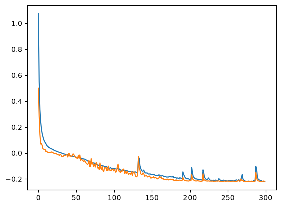
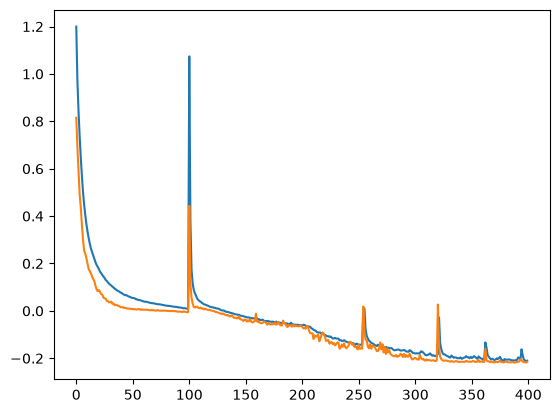
Our train and validation loss don't change much — 0.61 and 0.609 respectively.

This was a little surprising to me. I'd have guessed that positional information would be crucial to distinguish 91+1 from 19+1 and arrive at the right answer. After a few minutes of reading the literature on this, it turns out that thanks to the design of self-attention, tokens accumulate the context of everything that came before them over multiple layers. So for 19+1, the token 9 "knows" that 1 appeared before it, and over multiple layers that information gets richer and is carried forward until the final = token.

The decoding results look good:

('72+90=162#', True)
('3+50=53#',   True)
('90+68=158#', True)
('5+51=56#',   True)
('52+5=57#',   True)
('36+24=60#',  True)
('46+11=57#',  True)

and the model no longer makes the same mistakes as before on 2+3 and 3+8.

Keeping RoPE and continuing, now with tied embeddings.

Tied Embeddings

This was by far the easiest change, and it also reduces our parameter count.

Tying the embeddings means we don't have separate embedding and unembedding matrices. unembed = embed.T, and when we take the dot product x @ unembed, we assign a logit to each vocab token and the maximum is our prediction.

Apart from being beautiful, tied embeddings are also more sample-efficient, since the embedding matrix gets two gradient updates per batch instead of one.

We can see that from our loss curves below.

We get our lowest train loss of 0.58 and validation loss of 0.603.

Sample decodings:

('72+90=162#', True)
('3+50=53#',   True)
('90+68=158#', True)
('5+51=56#',   True)
('52+5=57#',   True)
('36+24=60#',  True)
('46+11=57#',  True)

Tied embeddings tend to be more popular in smaller models because as the model shrinks, the embedding matrix takes up a larger proportion of total params.

Masked Loss

Going back to our data split and staring at the loss function, you'll notice that we make a prediction for every token in the input. That means, for 1+1=2#, the first token is expected to output +, and then 1+ is expected to output 1. This is kind of nonsense, since we're expecting the model to predict what the next operand itself is going to be.

That's not a useful signal, mostly because the model can't possibly guess what the next operand will be. On the other hand, the model is going to see all possible values in the training data anyway, so perhaps this helps it generalize faster? Either way, since we average the loss across the full sequence, this is dragging our reported loss up. A cross-entropy loss of 0.60 corresponds to the model assigning roughly e^(-0.60) ≈ 0.55 probability to the correct token at each position. We can drive this lower by masking all predictions until the = sign and only penalizing the tokens that represent the answer.

Implementing this required some other changes to our train_step and loss functions to play well with jax.jit() and scan.

EQ_ID  = stoi["="]
PAD_ID = stoi["#"]

def answer_mask(x: jax.Array) -> jax.Array:
    """1 at positions whose y is an answer/stop token, 0 elsewhere.
    Scored region = from the `=` token through the last non-pad input."""
    seen_eq = jnp.cumsum(x == EQ_ID, axis=-1) > 0
    not_pad = x != PAD_ID
    return (seen_eq & not_pad).astype(jnp.float32)


def loss_fn(params, batch, key, is_train=False, loss_type="masked"):
    x, y = batch
    _, logits = forward(params, x, key, is_train)
    logp = jax.nn.log_softmax(logits, axis=-1)
    nll  = -jnp.take_along_axis(logp, y[..., None], -1).squeeze(-1)   # (B, T)

    if loss_type == "per_token":
        return nll.mean()

    if loss_type == "masked":
        mask = answer_mask(x)
        return (nll * mask).sum() / jnp.maximum(mask.sum(), 1.0)

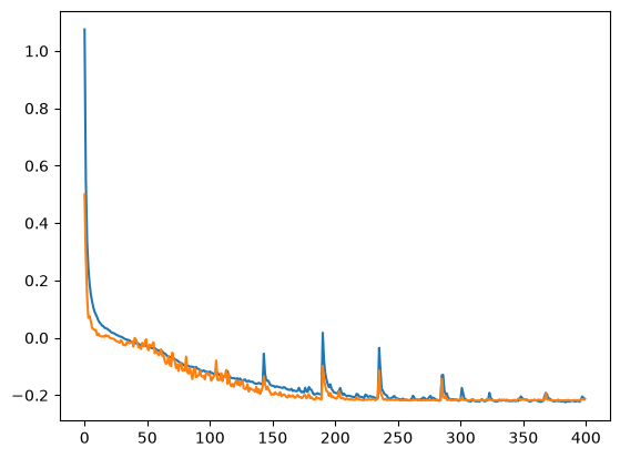
Ignoring the spikey loss curve, this result seemed very suspicious to me. Not only do we achieve a loss of 0.00001 on validation, the validation loss is significantly lower than training. I went back through my code a few times to make sure I wasn't leaking test data into the training loop.

In conclusion, after masking the loss to only score the answer tokens, we've essentially solved 2-digit addition. So why the stark gap between training and validation loss? The answer is Dropout — which zeros out random entries along d_model during training but not at eval time.

Limit to MAX_OPERAND = 50

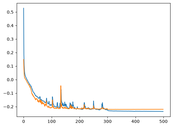
As an additional check on generalizability, we'll train the model on sequences with MAX_OPERAND = 50. Both the train and validation set use this data, and then we test the model on sequences outside the range, like 50+1=, to see whether the model is learning true addition, or just memorizing the value combinations it has seen.

We achieved a similarly low loss close to 0 on both train and validation sets.

But to my disappointment, when we test on out-of-distribution data, the model struggles:

('50+1=15#', False)
('50+2=15#', False)
('50+3=18#', False)
('50+4=45#', False)
('50+5=50#', False)
('50+6=41#', False)
('50+7=4#',  False)
('50+8=4#',  False)
('1+50=15#', False)
('2+50=25#', False)
('3+50=35#', False)
('4+50=45#', False)
('5+50=40#', False)
('6+50=41#', False)

Another benefit of training on calculator data is that we can trivially generate out-of-distribution sequences to probe what the model has actually learned.

Summary and Next Steps

We started with a barely-working SGD baseline (train/val loss 1.16 / 1.04, decoded answers were mostly wrong) and ended with a 0.5M-param transformer that essentially solves in-distribution 2-digit addition. Each component pulled its weight — though not always in the way I expected:

• Adam was by far the biggest single win — more than half of the total loss reduction came from swapping the optimizer.
• RoPE barely moved the loss number. The model was already picking up positional structure through stacked self-attention. It still helped on specific failure cases like 2+3 and 3+8.
• Tied embeddings matched the un-tied loss while cutting parameters — free win, especially at this scale where embeddings are a big slice of the param count.
• Masked loss turned out to be the most clarifying change. Once we stopped penalizing the model for predictions it could never get right (the operand tokens), validation loss collapsed to ~1e-5 and the train/val gap exposed dropout as the real source of "noise" in the reported numbers.
• OOD generalization is hard. The MAX_OPERAND = 50 experiment was the humbling moment — perfect in-distribution accuracy, near-random behavior the moment we ask it for 50+1. Low loss is not the same as learning addition.

There are three directions I want to push next:

1. Data scale-up — bump MAX_OPERAND to 999, add subtraction and multiplication, and see whether more data alone closes the OOD gap or just produces a better memorizer. Sequence length grows too, so this is also a test of how cleanly the data pipeline (vmap + scan) holds up at 100x the sample count.
2. Model scale-up — sweep d_model and num_layers from 0.5M → 2M → 5M → 10M params and plot loss vs. params at fixed data. The interesting question is whether OOD accuracy is a smooth function of scale, or whether there's a threshold beyond which the model "gets" the algorithm.
3. Profiling — measure step time, compile time, and HBM usage. Specifically: how much does scan vs. unrolled actually save us on compile time? What does the trace look like once we have a non-trivial model? Where are we sitting on the roofline at the 10M scale? This is the part of JAX I most want to build intuition for, and a small model is the right place to start since each iteration is fast.

I'll cover each of these in follow-up posts.